Adaptive multilevel MCMC sampling.

Developing an MCMC algorithm for efficient Bayesian inference in multilevel models

Funding. Alan Turing institute

Developing and implementing a new method called Multi-Level Delayed Acceptence (MLDA) to drastically accelerate inference in many real-world applications where spatial or temporal granularity can be adjusted to create multiple model levels.

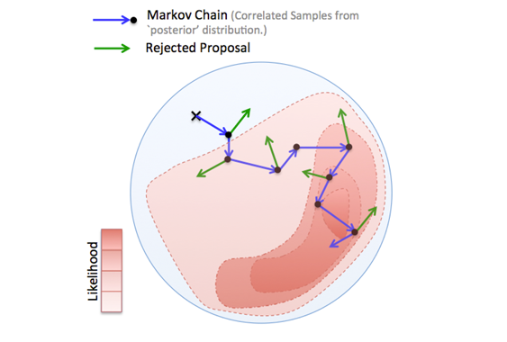
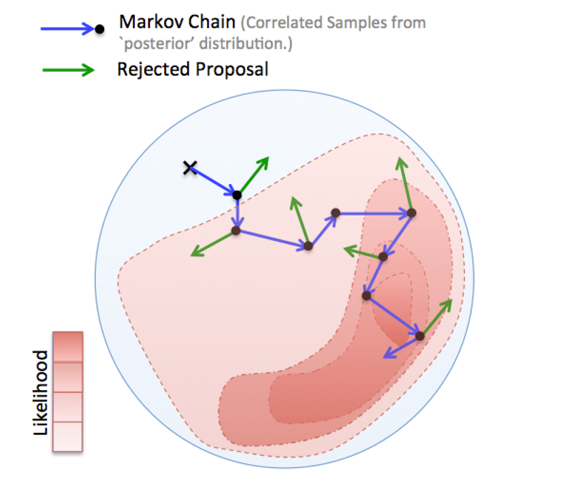
Sampling from a Bayesian posterior distribution using Markov Chain Markov Chain Monte Carlo (MCMC) methods (Fig. 1) can be a particularly challenging problem when the evaluation of the posterior is computationally expensive and the parameter space and data are high-dimensional. Many MCMC samples are required to obtain a sufficient representation of the posterior. Examples of such problems frequently occur in Bayesian inverse problems, image reconstruction and probabilistic machine learning, where calculating the likelihood depends on the evaluation of complex mathematical models (e.g. systems of partial differential equations) or large data sets.

Fig.1 - An MCMC algorithm drawing samples from a 2D distribution. In each step a proposed sample is generated and it is either accepted (blue) or rejected (green). If rejected, the previous sample of the chain is replicated. Samples occur more frequently in areas of high probability.

This project has developed and implemented an MCMC approach (MLDA) capable of accelerating existing sampling methods, where a hierarchy (or sequence) of computationally cheaper approximations to the 'full' posterior density are available. The idea is to use samples generated in one level as proposals for the level above. A subchain runs for a fixed number of iterations and then the last sample of the subchain is used as the proposal for the higher-level chain (Fig. 2).

Fig .2 - Three-level MLDA: For each step of the fine chain, a coarse subchain is created with length 3. The last sample of the subchain is used as a proposal for the fine chain.

The sampler is suitable for situations where a model is expensive to evaluate in high spatial or temporal resolution (e.g. realistic subsurface flow models). In those cases it is possible to use cheaper, lower resolutions as coarse models. If the approximations are sufficiently good, this leads to good quality proposals, high acceptance rates and high effective sample size compared to other methods.

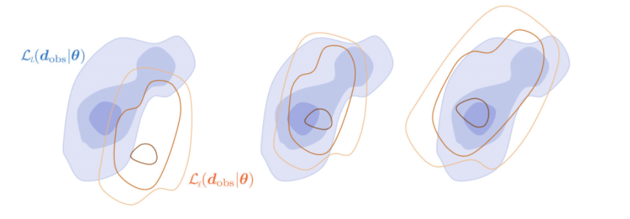
In addition to the above main idea, two enhancements to increase efficiency have been developed. The first one is an adaptive error model (AEM). If a coarse model is a poor approximation of the fine model, subsampling on the coarse chain will cause MLDA to diverge from the true posterior, leading to low acceptance rates and effective sample size. The AEM corrects coarse model proposals employing a Gaussian error model, which effectively offsets, scales and rotates the coarse level likelihood function (Fig. 3). In practice, it estimates the relative error (or bias) of the coarser model for each pair of adjacent model levels, and corrects the output of the coarser model according to the bias.

Fig 3 - Adaptive Error Model (AEM): When the coarse likelihood function (red isolines) is a poor fit of the fine (blue contours), AEM offsets the coarse likelihood function (middle panel) using the mean of the bias, and scales and rotates it (right panel) using the covariance of the bias.

The second feature is a new Variance Reduction technique, which allows the user to specify a Quantity of Interest (QoI) before sampling, and calculates this QoI for each step at every level, as well as differences of QoI between levels. The set of QoI and QoI differences can be used to reduce the variance of the final QoI estimator.